It’s been a little while since I last posted, as the team and I at Enso have been hard at work on the new version of the app. We released version 2025.1 a couple of weeks ago with a huge number of new features and improvements.

As anyone live in the UK will know, it has been a very dry spring so far. As I write this, it is another beautiful sunny day in London, and the forecast is for more of the same. I wanted to use Enso to take a look at the rainfall data for the UK. I will use the UK Met Office data, which is available on their Climate Data page. The specific data I will be looking at is the UK monthly rainfall data starting from 1836.

Fetching and Parsing the data

Looking at the data, it is clear that it is in a fixed-width format. The first five lines are the header, and the rest of the data is in a fixed-width format. Let’s bring this data into Enso and see what we can do to parse it. Currently, fixed-width native support is only in the nightly build of Enso, so I will show how to do it using the current release version. The nightlies are available from our GitHub repository here.

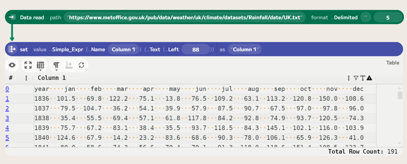
The Data.read command is used to read data into Enso. It can read from files or URLs. In this case, it downloads the data from the Met Office website and reads it into Enso. The data is identified as plain text and read into Enso as Text. We can, however, tell it to read it as a delimited file and then skip the header rows.

To do this, choose the Delimited option in the format command. This will allow us to specify the delimiter, which in this case is {none} as it is not delimited. We can also select the number of header rows to skip, which is 5. The data is then read into Enso as a single-column Table. As we are only interested in the monthly data, use a set component to take just the first 88 (4 for the year, 7 for each month) characters of each value (using Text Left).

Now, we want to split into columns. I will use regular expressions here as that is my favourite way of doing such things. The tokenize_to_columns function takes a column and a regular expression and splits the column into multiple columns. If there is a marked group in the regular expression, it will be used as the value, and the other parts will be discarded. The expression I am using is \s{0,7}(\S+). This will match any whitespace (up to 7 spaces) followed by a non-whitespace sequence (the data we want).

I then do a couple more transformations to the data:

1. Use the first row as the column names.
2. Replace empty values with Nothing.
3. Parse all the values.

Comparing year by year

Now that we have the data in a nice format, we can start to do some analysis. I want to change the data to a row-based format with columns for year, month and rainfall. A transpose component will rotate the data, and then we can convert the month name to a season. I created a lookup table (using Table.input) to convert the month names to numbers and seasons. I then use a merge component to join the data with the lookup table. This gives us a table with the year, month, season and rainfall values.

As December is in the winter, we need to add a season year column to the data. This is the year unless it is December, in which case it is the following year. Using a set component with an expression of if [month]="dec" then [year]+1 else [year] to make the new column.

Finally, in preparing the data, need to add a row for May 2025, as this is not currently in the monthly data. Based on the article, the average for Spring 2025 is 80mm, so for May this comes out as just 2.7mm. Using another look up table and merge component we can update this value and then filter out the future rows (where the rainfall is Nothing).

To create the yearly data, filter down to the interesting months (here March, April and May). Using another lookup table linked to a filter where month Is_In allows you to do this easily. Then aggregate by season year, creating the total rainfall for each year.

Computing the average of the previous 20 years

One of the new features in the 2025.1 release is the ability to use Table.offset to access previous rows in a table. This allows us to easily compute a rolling average. It can be used as its own component or within an expression. You do need to ensure that the table is sorted first, but this is done easily using a sort component (you can specify the ordering in the offset component as well).

First, we use a running component to compute a new running total of rainfall since 1836. To then get the value from 20 years ago, use the Table.offset function with n set to -20. One of the really powerful features of Enso is that everything can be passed into parameter to dynamically configure components. So we can have the value of the number of years as its own component. This allows us to change the number of years we look at easily.

As offset needs a negative value, computing the average will also need the number of years, so first, multiply the number by -1. The offset function returns a table with an additional column with the shifted values, with a name of offset([running], -20, ..Nothing). As this depends on the number of years, a rename_columns function is needed to normalise the name to running_start.

Finally, to compute the average, a set component is used. Showing some of the power of this component, you can combine Simple_Expression and expressions. Let’s take a look at the expression: offset([running],-1)-[running_start]. The first part, offset([running],-1), gets the previous value of the running total by using a offset inline of the expression. The second part, - [running_start], subtracts the value from 20 years ago. This gives us the total rainfall for the last 20 years.

The Simple_Expression is then used to divide this value by the number of years to get the average. The final result is a table with the year, month, season and rainfall values, as well as the average rainfall for the previous 20 years for each row.

Calculating a z-score

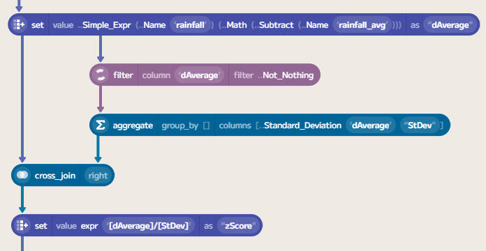
To compute the deviation from the average, we can subtract the average from the current value. This is done using another set component. To calculate the z-score, we need to divide this value by the standard deviation. The z-score measures how many standard deviations a value is from the mean. A z-score of 0 means that the value equals the mean, while a z-score of 1 indicates that the value is one standard deviation above the mean.

You could compute a rolling standard deviation similarly to the rolling average above. However, for my analysis, I decided just to compute this over the entire dataset. This is a standard computation on the aggregate function. To attach this to the data, a cross_join will perform a Cartesian product of the two tables.

Finally, we can compute the z-score using a set component with the expression [dAverage]/[std_dev].

Displaying the data

Next, we can filter the rows to remove those without a z-score. These will be the first 20 years of data, as we are using a 20-year rolling average.

To pick the columns we want to display, use a select_columns component. In this case, keeping season_year, rainfall, rainfall_avg and zScore.

Enso can show data on a scatter plot, which is a great way to visualise the data. If you add a color column, you can use this to colour the points. In this case, I used the zScore column to colour the points when more than two standard deviations below the average.

This gives a nice visualisation of the data, showing the years with extreme rainfall, either very high or very low. 2025 stands out as an extremely dry year, being more than three standard deviations below the average of the last 20 years.

The table below shows the years outside two standard deviations:

Year	Rainfall	20yr Average	Z-Score
1862	284.3	176.7	2.50
1903	285.4	187.7	2.27
1913	311.4	207.0	2.43
1920	307.9	212.1	2.23
1947	326.8	180.7	3.40
1963	280.1	188.0	2.14
1967	294.5	195.7	2.30
1979	327.1	206.4	2.81
1986	313.8	211.4	2.38
2024	301.7	210.0	2.13
2025	80	213.3	-3.10

Conclusion

This is a simple example of how to use Enso to analyse data. The new features in 2025.1 make working with data and experimenting easy and quick. If you would like to download the completed workflow you can here.

While this is not a deep analysis, the flexibility and control of parameters and the live re-evaluation of results make it an excellent tool for examining historical data. This gives you a taste of what is possible with Enso and how easy it is to work with data. Please let me know in the comments below if you have any questions or comments.

If you want to try Enso, you can download the latest version from our website. We also have a community forum where you can ask questions and share your experiences with other users.