Some members of the team building Enso decided to try and tackle last year’s Advent of Code using the language and see how far we could get. I’ve previously tried solving Advent of Code in Alteryx and was personally interested to know whether it is easier or more challenging with what we are building.

For those not familiar with the Advent of Code, every year Eric Wastl creates a set of 25 programming puzzles posted once a day over December. Each puzzle has two related parts with an example set of values and the expected result based on these. Often, the second part is a more challenging extension of the first part. Generally, there should be a solution that can complete within a few seconds (although we didn’t always find that one!).

This post summarises a few of the puzzles we tried and some of the challenges we faced, giving the views and experience of myself, Jaroslav Tulach, and Radosław Waśko of us trying to solve them.

Jaroslav’s Experience with Day 1 – Calorie Counting

• https://adventofcode.com/2022/day/1

Initial tasks of Advent of Code are usually quite simple. That is great, especially when starting with a new language or an IDE. As such, let’s look at the Calorie Counting task and how it can be solved with Enso and its IDE. I’ll do my best to share what I learned while going through the puzzle. I was not new to the Enso language – e. g. it wasn’t a problem to express the algorithm. However, I usually coded Enso in a text editor. This time I wanted to taste the real Enso IDE experience.

Problem #1 – how do I read a file? When you create a project, you get an src directory. However, you can also make a data directory sibling and put the associated data files there. You can then reference that directory as enso_project.data in your code. Reading a text file is then simple as

enso_project.data/"aoc1-test.txt" . read

Problem #2 – working with the textual file requires you to split the text into lines. Great, there is .lines function. But then there are groups of lines waiting to be processed. My original solution was just .fold over the lines and pass in a Pair of two numbers. However, there is a much nicer solution: operator1.split '\n\n' – split the text on two new lines! Then one gets the needed groups easily.

Problem #3 – converting the text lines to numbers. It is as simple as _.map Integer.parse – however, I learned a handy trick. You can collapse a graph of nodes into a new function. You can then use it in multiple places. Not just that, when double-clicking on the function name, you tell the Enso IDE to open up the collapsed part, and you can refine it and test it with input values. That’s cool as it allows one to keep the program clean, focused on individual tasks, and nicely organized inside a single project.

Problem #4 – is to do some statistics on the obtained data. If you are like me, you just do some arithmetic, but the cool kids (those who know all the Enso libraries) use Statistic library functions. Then it is just about requesting Statistic.Maximum, or Statistic.Sum. Nice, powerful, and easy to obtain the desired results.

The ‘Calorie Counting’ was a simple task, but it opened the door for me to the Enso IDE, its concepts, and the power of the libraries it offers. I recommend trying this simple task yourself. It is fun, and it is worth it!

My Experience with Day 8 – Treetop Tree House

• https://adventofcode.com/2022/day/8

So by day 8, we were more into the swing of it, and the internal competition had heated up. The timezone disadvantage of living in the UK was showing, and those early risers were getting solutions published before I was even awake! The first week of puzzles led to various library improvements and stability fixes that made working in the IDE more pleasant and quicker.

Again the first challenge is loading the data and shaping it into something we can work with:

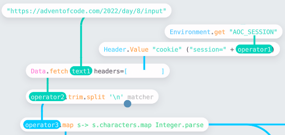
I chose to fetch the data directly from the website using Data.fetch. This API reads the URL, and if in a format Enso recognizes will automatically parse it. In this case, the data is just text. I wanted to parse the text into a 2D vector of integers, which is easily accomplished by breaking it into lines (using .lines) and then parsing each character (the .map s → s.characters.map Integer.parse).

The next task is to find how many trees are visible outside the grid. Taking just the horizontal scan, I built a small function (using the approach Jaroslav describes above by grouping nodes):

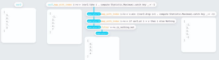
The function works by computing the maximum height from both ends of the vector to the current point and seeing if the current is higher. It then gathers the indices of visible trees. The view shown is the expanded function showing how you can trace the computation through. var2 is the input to the method, and it is easy to change the values and test the process from the parent workflow.

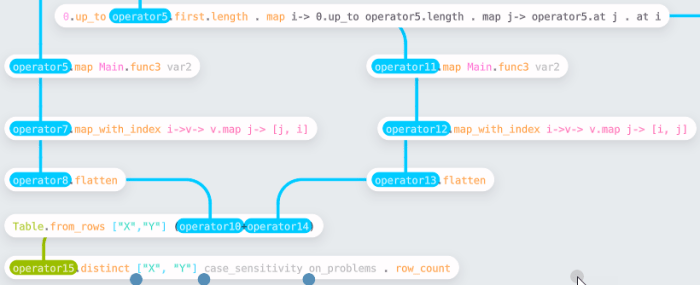
Having built the row process (called Main.func3 in the workflow), this can then be run on columns by transposing the input dataset. Finally, having gathered the complete set of coordinates, we need to make a unique set to find the count. I chose to do this by converting to a table (using Table.from_rows) and then using the .distinct function.

Part 2 was a straightforward adjustment to the process, looking out from a tree rather than looking in.

Since building this workflow, we have added the ability to compute running statistics which would have made these computations easier. Likewise, the issue we had at the time with Vector.distinct has been resolved, so the need to convert to a table is removed.

Radosław’s Experience with Day 12 – Hill Climbing Algorithm

• https://adventofcode.com/2022/day/12

In this puzzle, I was given a height map of the terrain, and I had to find the shortest route to a particular endpoint, only being allowed to go up at most 1 unit on each step. This is a classic task for a BFS algorithm, and starting to write it, I decided it may be easier to write the main loop itself in text mode. So I did just that:

## A helper that updates a 2d array,
   setting the entry at coordinates [vx, vy] to the value `val`.
set visits vx vy val  =
    operator8 = visits.map_with_index y-> v->
        if y == vy then (v.map_with_index x-> e-> if x == vx then val else e) else v
    operator8

## Checks if the new coordinate was already visited or is out of bounds
   (we also treat it as `visited`, to not go outside the map).
is_visited visits x y =
    if (x < 0) || (x >= visits.first.length) then True else
        if (y < 0) || (y >= visits.length) then True else
            visits.at y . at x

## The core BFS loop.
   The looping is done by tail-recursive calls.
bfs heights visits queue dists =
    if queue.is_empty then dists else
        q = queue.first
        x = q.at 0
        y = q.at 1
        d = q.at 2
        n1 = [[x+1, y], [x-1, y], [x, y+1], [x, y-1]]
        n2 = n1.filter v-> is_visited visits v.first v.second . not<
        height p = heights.at p.second . at p.first
        n3 = n2.filter p-> (height p) <= (height [x, y] + 1)
        next = n3.map v-> v+[d+1]
        visits2 = next.fold visits (acc-> p-> set acc p.first p. second True)
        dists2 = next.fold dists (acc-> p-> set acc p.first p.second (d+1))
        queue2 = queue.drop 1 + next
        @Tail_Call bfs heights visits2 queue2 dists2

## Prepares and runs a BFS from the given start point.
start_bfs start heights visits =
    visits2 = set visits start.first start.second True
    dists = visits2.map v-> v.map x-> if x then 0 else Number.positive_infinity
    bfs heights visits2 [start+[0]] dists

My function gets a starting point, a 2d array of integers representing the height map, and another 2d array of booleans representing the visited points. It returns a 2d array of integers representing the distances from the starting point to each point in the height map. It relies on two small helper functions that make the code more readable.

With these tools in my arsenal, I could return to the IDE and finish the job.

I tried to be fancy and forced Data.read to use a Delimited format to load a single-column table that I later converted into a vector. I could have read it as a regular text file and used the .lines split as my predecessors.

I’ve split each line into characters, replacing ‘S’ and ‘E’ with the letters corresponding to their heights (using a doubly-nested Vector.map). Then, I could use the ASCII representation (.utf_8 returning the byte value for a character) to generate a 2d array representing our input height map. Another doubly-nested map allowed me to create a 2d array of booleans representing the visited points – initialized as False everywhere.

I also needed to find the start and end points on the map. I’ve done so for the starting point and used the group tool to create a helper that I could then also use for the endpoint:

## Finds the 2d coordinates of the first occurrence of the given character in
   the array of strings.

   The first coordinate corresponds to the index of the string at which
   the character is found, and the second coordinate corresponds to
   the index of the string in the array.
find_location operator2 text1 =
    operator3 = operator2.map_with_index ix-> elem-> [elem.locate text1, ix]
    operator4 = operator3.filter v-> v.first.is_nothing.not
    operator5 = operator4.first
    operator6 = operator5.first.start
    operator7 = operator5.second
    var1 = [operator6, operator7]
    var1

Now, I could finally run the BFS I’ve shown above and get back a map of distances from the starting point to each point on the map. From this, I just had to read the distance to the selected endpoint.

Adapting the solution for Part 2 was relatively simple: I reversed the BFS, now starting at the end point E. To make this work, I had to adjust the condition to check if I can move between two adjacent squares to:

- n3 = n2.filter p-> (height p) <= (height [x, y] + 1)
+ n3 = n2.filter p-> (height p) >= (height [x, y] - 1)

With that, I’ve found all points on the height map that have height a and read their distances to E. Finally, I used Vector.compute to find the closest one (Statistic.Minimum). Having successfully got the second star, I celebrated finishing the task for the day.

However, Enso also has some abilities to visualize data, so I thought it was worth using these capabilities to show the height map and the distance map generated from it. I added a simple helper function that converts a 2d array of numbers into an Enso Table with the correct columns for the heatmap visualization.

When I switched to the real input data, the visualization did not look as nice. With a small change, it was easy to use the scatter-plot visualization that shows a sample of the dataset and is better suited for bigger datasets, allowing me to get a better view of what the height map in the actual input looked like:

The workflow was slightly adapted to work with the newer version of Enso; the changes were minimal – vector.tail needed to be replaced with vector.drop 1, and Data.read_file is now Data.read.

Conclusion

Using the IDE daily to solve these puzzles rapidly drove the development and improvement of both it and the libraries. We added various new features and corrected many problems and bugs we found along the way. Some highlights are listed below:

• Ability to drop a file on the IDE and have it parsed and ready to use.
• New Data.fetch API to retrieve and parse data from the web.
• Function to compute running statistics (for example, total) across a Vector.
• Overhauled and enhanced JSON support.
• Stabilized the visualization of data within the IDE.

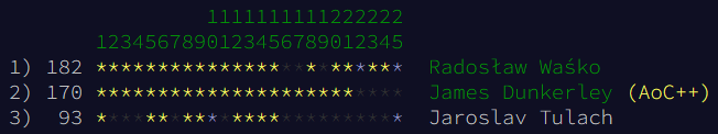
In the end, we managed to solve virtually every puzzle. We even automated posting a scoreboard of how we were doing to our discord conversation every day so the whole team could see.

Enso, as a general-purpose programming language, has grown significantly over the last year – solving the challenges showed this. Compared to solving similar problems in previous years within Alteryx, I found that some were much more straightforward and others harder (giving us some hints on what we need to fix and improve!). The IDE and API improvements over December made the solving experience smoother and more pleasant.

Next year, we look forward to trying it again with a more open competition with the community.