In this post, I will use the results from my last post to review how each category has performed against the sales targets the company has set.

The completed workflow from that post can be downloaded from GitHub.

The sales targets are stored in a JSON file, so they must first be parsed and then joined to the results from the last post. The raw JSON file can be downloaded from GitHub. Based on the 2014 data, they have category-level monthly targets from 2015 until 2017.

Downloading the Sales Targets

Let’s take a look at the JSON file:

{
    "Furniture": { 
        "2015": [5000,2000,19000,10000,8000,11000,11000,10000,27000,10000,26000,23000],
        "2016": [5000,2000,20000,10000,8000,12000,12000,10000,29000,10000,27000,24000],
        "2017": [5000,2000,22000,11000,9000,13000,13000,11000,31000,11000,29000,25000]},
    "Office Supplies": { 
        "2015": [5000,2000,19000,9000,8000,11000,11000,9000,27000,9000,25000,22000],
        "2016": [5000,2000,20000,10000,8000,11000,11000,10000,28000,10000,26000,23000],
        "2017": [5000,2000,21000,10000,9000,12000,12000,10000,30000,10000,28000,24000]},
    "Technology": {
        "2015": [5000,2000,19000,10000,8000,11000,11000,10000,27000,10000,26000,23000],
        "2016": [5000,2000,20000,10000,8000,12000,12000,10000,29000,10000,27000,24000],
        "2017": [5000,2000,22000,11000,9000,13000,13000,11000,31000,11000,29000,25000]}
}

Each category is listed as a key in the JSON object. The value for each category is another JSON object, with the years as keys and the sales targets as arrays. The first task is to load this into Enso. There are multiple ways to read data from a URL in Enso; a straightforward option is the Data.fetch method:

This method will download from the specified uri. The other parameters are optional, but let’s go through them. The method argument specifies the HTTP verb used – by default, GET is used; however, you can choose another. Please note that only verbs are allowed, which should not change things on the server. There is a Data.post method that accepts the other ones.

The headers argument specifies any HTTP headers you want to send with the request. These are passed as a Vector of pairs of Text values. For this request, there is no need to specify any headers.

Finally, the try_auto_parse_response controls how Enso handles the response from the server. If true (the default), Enso parses the body based on the Content-Type header. If false, then the reply will be returned as a Response object. In both cases, a data flow error will be returned if the status code indicates an error (i.e., not 200 – 299).

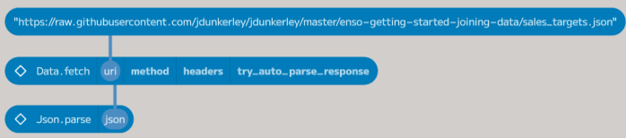
In this case, we want to parse the response as JSON, so leave the default value of true for try_auto_parse_response. However, the returned value is a Text value, as GitHub returns the Content-Type as text/plain. The Json.parse method can be used to convert this.

Working with JSON

One of Enso’s strengths is the ability to use a variety of programming languages within a project. Most functions are written in Enso’s native language, but other languages are also used. For example, the Json.parse method is written principally in JavaScript. The returned object is a JS_Object, a wrapper around an underlying JavaScript object, which works like any other Enso object. For example, the field_names method gets all the keys of the object:

In this case, the goal is to convert the JS_Object into a table. The Table.from_objects function will change various things, including JS_Object, into a table.

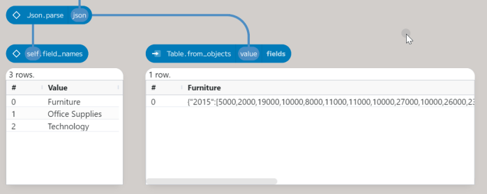
Each field within the object becomes a column. However, in this case, the categories should be rows.

The Table.transpose method converts a column-based table (like the result above) to a row-based one. You can supply an attribute_column_name to control the output name, in this case, Category. I’ll cover the other parameters below. The result is a table with two columns – Category and Value. The Value column contains the JS_Object for each category. The expand_column method allows spreading these objects out over a set of columns:

The first parameter is the column name to expand (the column parameter). The second argument, fields, can optionally provide a set of names to extract from each object (this is also the case for Table.from_objects). If not set, then a union of all fields is produced. Finally, the prefix parameter controls adding a prefix to new column names. By default, it will add the name of the source column, but in this case, just the value is needed. Now, back to a second transpose:

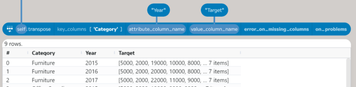
This time, a key_column entry is needed to keep the Category as a column. You can specify any number of columns which should not be transposed. The value_column_name allows us to change the output from Value to Target. Finally, also set the attribute_column_name as Year. The result is a table with three columns – Category, Year, and Target. The Target column contains the sales targets for each month as a Vector, so the next step is to expand this into rows (using the expand_to_rows method) and then finally add a Month column (using a row number function):

The expand_to_rows column’s first argument again specifies the column to work upon. In this case, if a cell contains a set of values (such as a Vector), it is expanded to new rows, each having a single value from the set, with the values from the other columns repeated for each new row added. The current row is added to the output table if the cell is a single value. The second parameter (at_least_one_row) controls whether to add a row for an empty Vector; if False (the default), these rows are dropped; if True, then the current row, with the input cell replaced with Nothing, is added.

The add_row_number function allows the creation of an index column. By default, this will be called Row and start numbering from 1. The name parameter allows changing the output name. The initial value and increment can be set using the from and step parameters. The following two options enable adding a grouping (in this case, by Category and Year) and finally allow for applying an ordering if desired.

The final process for downloading and reshaping the sales targets looks like this.

Joining the Data

The targets are now easy to work with and can be joined to the results from the previous post. Dragging out from the results and adding a join node looks like:

The first argument, right, takes a table to join with the self table. In this case, connect the output from the restructure process to this. The second argument, join_kind, controls the type of join to perform. The default is a left-outer join – all rows from the left input (self) and the matching rows from right are returned. Enso supports the following join types:

	Join Kind	Left Rows	Right Rows	Columns Returned
	Left Exclusive	All	Non-Matching	Left Only
	Left Outer	All	Matching	All
	Inner	Matching	Matching	All excluding equality columns
	Right Outer	Matching	All	All
	Right Exclusive	Non-Matching	All	Right Only
	Full Outer	All	All	All

Most of these joins are the same as you get in SQL. The Left Exclusive and Right Exclusive joins are additions that allow you to get the rows that were not successfully joined. These can be hugely useful to ensure no data is lost. Another feature to note is that the join_kind also determines the set of columns returned. For example, the Left Exclusive join only returns columns from the left input because no rows from the right input matched. The Inner join excludes the equality columns, as they are the same in both inputs. For this example, the Inner join will work perfectly.

The following parameter, on, specifies how to match the rows between the inputs. By default, it will attempt to match the first column in the left input with a column in the right with the same name. It takes a Vector of Join_Condition, which allows either an Equals condition or a Between (the left table contains a value between two columns in the right).

The right_prefix argument adds a prefix to clashing column names from the right table. The default value, "Right ", is added if a column exists in both tables. You can specify whatever prefix you wish to use. If the name is still not unique, a number is added to the end, and a warning is raised. The on_problems parameter works as in other functions to handle how warnings are dealt with.

In this case, the Category, Year, and Month values must be equal. Add three Equals conditions to the on parameter and then choose the name from the dropdown on each left parameter. By default, the right parameter will be the same as the left one, but you can change this if needed (though the current UI does not support a dropdown on the right side). Once done, an error will be shown:

The error is because the Year column is a Text value in the restructured table but an Integer in the results table. The parse function can be added before this join node to convert the Year column to an Integer (there is no need to select a type as it will automatically determine all are Integer values):

Creating the Summary Table

The table now has Target and Sum Sales (from the previous post) columns; the next step is to add a column with the difference between the two (using the set method):

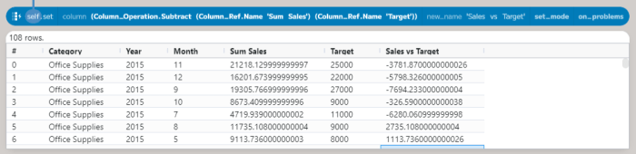
First, using the cast to convert the new column to Integer values removes the decimal places. This can then be fed into the cross_tab method, which can be used to create a summary table.

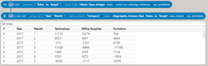
The first argument, group_by, specifies a set of columns to group the data by. In this case, the Year and Month columns are used. The second argument, name_column, tells the method where to get the new column names. The third argument, values, sets how to compute the value for each cell. The default is to count the number of rows in each group, but you can choose any aggregation function. In this case, the sum function adds the values in the Sales vs Target column.

One final step is to order the results Year and Month. The complete process of building the summary table looks like this:

Wrapping Up

In this post, we have looked at many powerful features in Enso for reading and restructuring data. Building on top of the methods introduced before, this time we have seen:

• Data.fetch: reading and parsing data from the web.
• Json.parse: parsing JSON data from a `Text“ value.
• Table.from_objects: converting objects into a table.
• Table.transpose: converting a column-based table to a row-based one.
• Table.expand_column: expanding a column of objects into multiple columns.
• Table.expand_to_rows: expanding a column of lists into multiple rows.
• Table.add_row_number: adding an index column to a table.
• Table.join: joining two tables together.
• Table.cross_tab: creating a summary table from a table.

The completed workflow from this post can be downloaded from GitHub. As always, I hope you will consider trying out Enso. If you have any questions, please join our Discord server or comment below.

I will take a break from this series for December to concentrate on solving Advent of Code in Enso, but more on that later in the week. I’ll be back in January with the next post in this series.